Quantum Regressor#
Quantum Doctor#
How to train a hybrid-quantum neural network to predict diabetes progression in patients.#
In this tutorial you will learn how to create a hybrid neural network, which utilizes a quantum regression layer as its output.
As our training dataset we will use a subset of the diabetes toy dataset available via scikit-learn.
Table of contents:#
import warnings
warnings.simplefilter('ignore')
Dataset preparation#
We can load our dataset via the load_diabetes method available from sklearn.datasets as it is one of the toy datasets provided by the library.
You might notice that the \(X\) values are already processed. This will save us time.
We will only use 200 samples from the 442 total, 100 for training and 100 for evaluation.
import pandas as pd
from sklearn.datasets import load_diabetes

diabetes = load_diabetes()

X = pd.DataFrame(diabetes.data[:200],columns=diabetes.feature_names)
y = pd.Series(diabetes.target[:200])
The diabetes dataset consists of 10 numeric variables: age, sex (2 possible values), body mass index (bmi), average blood pressure (bp), as well as results of six blood serum measurements (described on the sklearn dataset page).
X.head(5)
| age | sex | bmi | bp | s1 | s2 | s3 | s4 | s5 | s6 | |
|---|---|---|---|---|---|---|---|---|---|---|
| 0 | 0.038076 | 0.050680 | 0.061696 | 0.021872 | -0.044223 | -0.034821 | -0.043401 | -0.002592 | 0.019907 | -0.017646 |
| 1 | -0.001882 | -0.044642 | -0.051474 | -0.026328 | -0.008449 | -0.019163 | 0.074412 | -0.039493 | -0.068332 | -0.092204 |
| 2 | 0.085299 | 0.050680 | 0.044451 | -0.005670 | -0.045599 | -0.034194 | -0.032356 | -0.002592 | 0.002861 | -0.025930 |
| 3 | -0.089063 | -0.044642 | -0.011595 | -0.036656 | 0.012191 | 0.024991 | -0.036038 | 0.034309 | 0.022688 | -0.009362 |
| 4 | 0.005383 | -0.044642 | -0.036385 | 0.021872 | 0.003935 | 0.015596 | 0.008142 | -0.002592 | -0.031988 | -0.046641 |
The target variable is a quantitative measure of diabetes progression after one year.
y.head(5)
0    151.0
1     75.0
2    141.0
3    206.0
4    135.0
dtype: float64
As usual we will create the training and evaluation subsets using train_test_split
from sklearn.model_selection import train_test_split

X_train,X_test,y_train,y_test = train_test_split(X,y,test_size=0.5,random_state=42)
Model creation#
Quantum layer circuit#
A fairly simple QNN architecture will be used for the quantum layer, consisting of one input encoder applied at the beginning and end of the circuit and a RealAmplitudes block for the weights.
import numpy as np
# QNN library integrating with PyTorch
from qailab.circuit import build_circuit, RotationalEncoder, RealAmplitudesBlock
from qailab.circuit.utils import assign_input_weight

input_encoder = RotationalEncoder('x','input')
qnn_circuit = build_circuit(
    3,
    [
        input_encoder,
        RealAmplitudesBlock('weight'),
        input_encoder, # You can put the same block twice in different parts of the circuit. It will encode the same parameters
    ],
    measure_qubits=[0,1,2] # Measure all qubits
    )

qnn_circuit.assign_parameters(assign_input_weight(qnn_circuit,[1,2,3],np.random.randint(0,9,12))).draw('mpl')

Sequential neural network#
Our neural network will consist of two linear layers with ReLU activation functions, then a quantum layer, which outputs a single feature: the expected value of measurement from it’s circuit.
The expected value of a random variable can be expressed as \(E[X] = \sum_{i=0}^{n} P(X == X_i) * X_i\)
Given that our measurement bitstrings can be interpreted as integers, the expected value of a parameterized quantum circuit becomes \(E[X] = \sum_{i=0}^{n} |\braket{X_i|U(\theta)|0}|^2 * \text{integer}(X_i)\), where \(X_i\) is a given measurement bitstring.
Since we measure all 3 qubits in our QNN circuit, the expected value layer will output a value in the range of \([0,7]\). Our problem needs a higher range of numbers, therefore we will tell ExpectedValueQLayer to rescale the output.
# Neural networks libraries
import torch.nn as nn

from qailab.torch import ExpectedValueQLayer,QModel
from quantum_launcher.routines.qiskit_routines import AerBackend

qlayer = ExpectedValueQLayer(
    qnn_circuit,
    rescale_output=(0,350), # Max target value in dataset + a bit more.
    backend=AerBackend('local_simulator')
    )

sequential_net = nn.Sequential(
    nn.Linear(len(X.columns),64),
    nn.ReLU(),
    nn.Linear(64,qlayer.in_features),
    qlayer,

)

model = QModel(
    module=sequential_net,
    loss=nn.L1Loss(), # MAE loss
    optimizer_type='adam',
    learning_rate=0.001,
    batch_size=4,
    validation_fraction=0.1,
    epochs=20,
    metric="mse"
    )
Model training and results.#
Training#
To train our model we can simply call QModel.fit()
model.fit(X_train,y_train)
pass
100%|██████████| 20/20 [03:20<00:00, 10.00s/epochs, epoch=20, loss=47.6, mse=3.38e+3]
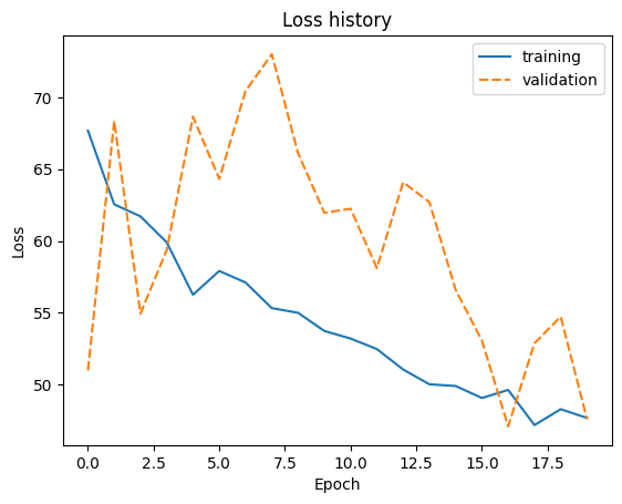
Below we can see how our model was performing during the 10 epochs of training.
import seaborn as sns
import matplotlib.pyplot as plt

sns.lineplot(model.loss_history)

plt.title('Loss history')
plt.ylabel('Loss')
plt.xlabel('Epoch')

plt.show()
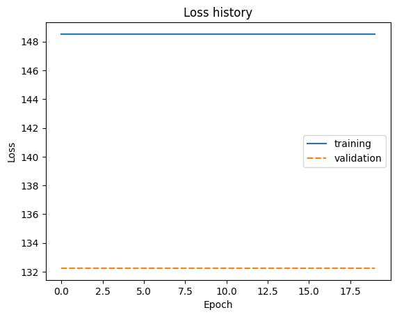
As a comparison we will also train a similar classical model.
sequential_net_classical = nn.Sequential(
    nn.Linear(len(X.columns),64),
    nn.ReLU(),
    nn.Linear(64,3),
    nn.ReLU(),
    nn.Linear(3,1),
    nn.ReLU()

)
model_classical = QModel(
    module=sequential_net_classical,
    loss=nn.L1Loss(), # MAE loss
    optimizer_type='adam',
    learning_rate=0.001,
    batch_size=4,
    validation_fraction=0.1,
    epochs=20,
    metric="mse"
    )
model_classical.fit(X,y)
pass
100%|██████████| 20/20 [00:02<00:00, 8.09epochs/s, epoch=20, loss=132, mse=97595.0]
import seaborn as sns
import matplotlib.pyplot as plt

sns.lineplot(model_classical.loss_history)

plt.title('Loss history')
plt.ylabel('Loss')
plt.xlabel('Epoch')

plt.show()
Model evaluation#
Let’s compare the performance of our models on the test dataset.
from sklearn.metrics import mean_absolute_error

classical_predictions = model_classical.predict(X_test)
quantum_predictions = model.predict(X_test)

print(f"Classical model error: {mean_absolute_error(classical_predictions,y_test)}")
print(f"Hybrid model error: {mean_absolute_error(quantum_predictions,y_test)}")
Classical model error: 152.19
Hybrid model error: 46.13027381896973